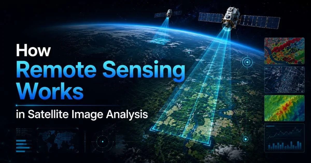
How remote sensing works in satellite image analysis is a question that sits at the foundation of modern geospatial science. Whether you're tracking urban sprawl, monitoring deforestation, or classifying agricultural patterns, understanding the mechanics behind remote sensing transforms raw satellite data into actionable intelligence. For GIS analysts and researchers, this isn't abstract theory.
It's the operational backbone of every project that relies on earth observation data. The technology has matured significantly over the past two decades, yet many practitioners still work with incomplete mental models of the full pipeline.
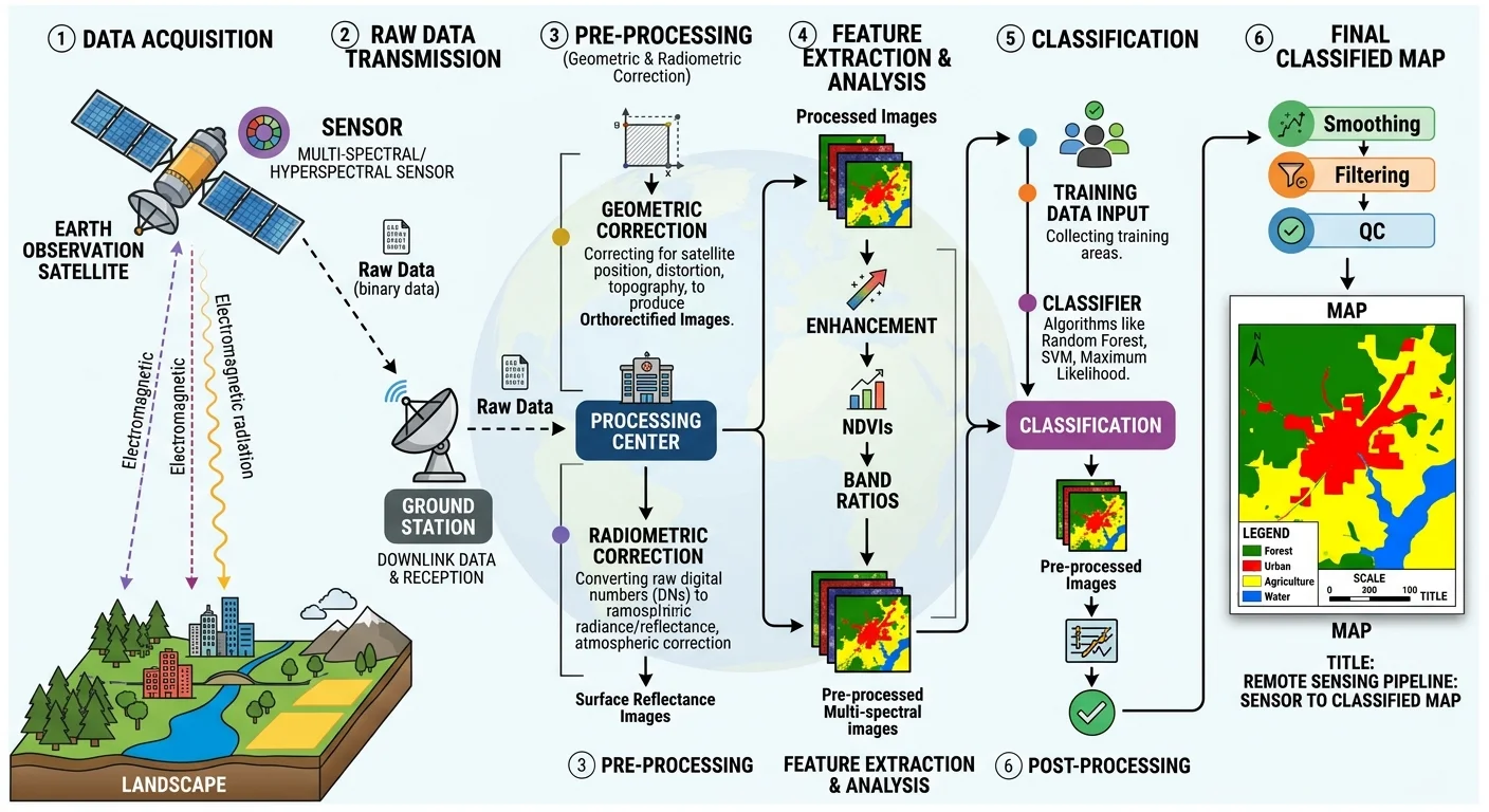
This guide walks through the process step by step, from sensor physics to final output, giving you a practical framework you can apply to your own satellite image analysis workflows. By the end, you'll have a clear understanding of each stage and how they connect.
Key Takeaways
- Remote sensing captures reflected or emitted energy across multiple spectral bands for analysis.
- Preprocessing steps like atmospheric correction directly determine the accuracy of your results.
- Band combinations and spectral indices reveal land patterns invisible to the human eye.
- Classification algorithms convert pixel data into meaningful thematic maps for decision-making.
- Validation against ground truth is non-negotiable for any credible remote sensing study.
Step 1: Understand Sensor Types and How They Capture Data
Passive vs. Active Sensors
Every remote sensing workflow begins with the sensor. Passive sensors, like those aboard Landsat 8 or Sentinel-2, detect sunlight reflected off the Earth's surface. They work well in clear weather and daylight conditions but struggle with cloud cover. Active sensors, such as Synthetic Aperture Radar (SAR) on Sentinel-1, emit their own energy pulses and measure what returns. This makes SAR invaluable for monitoring in tropical regions where persistent cloud cover would otherwise block optical observation entirely.
The choice between passive and active sensing depends on your project requirements. If you need fine spectral detail for vegetation health assessment, optical sensors are your best option. If you need consistent temporal coverage regardless of weather, or you're measuring surface deformation, SAR is the stronger tool. Many advanced studies combine both, a technique called data fusion, to overcome the limitations of either approach alone.
Why Spectral Resolution Matters
Spectral resolution refers to how finely a sensor divides the electromagnetic spectrum into discrete bands. Multispectral sensors like Sentinel-2 capture 13 bands, while hyperspectral instruments like PRISMA or AVIRIS record hundreds. More bands mean finer discrimination between materials. For example, distinguishing between two crop types that look identical in visible light often requires narrow bands in the shortwave infrared region. Understanding your sensor's spectral capabilities is the first step toward knowing what questions your data can actually answer.
Spatial resolution is equally important. A 10-meter pixel from Sentinel-2 is suitable for regional land cover mapping, but detecting individual buildings or small water bodies demands sub-meter imagery from commercial providers like Maxar or Planet. Temporal resolution, how often a sensor revisits the same location, determines whether you can track rapid changes. Sentinel-2 offers a 5-day revisit cycle, making it strong for time-series analysis of seasonal patterns across agricultural landscapes.
Step 2: Preprocess Your Satellite Imagery Correctly
Radiometric and Geometric Corrections
Raw satellite data contains distortions introduced by sensor electronics, platform motion, and Earth's curvature. Radiometric calibration converts raw digital numbers into physically meaningful values like radiance or reflectance. Without this step, comparing images from different dates or sensors produces misleading results. Most GIS analysts rely on metadata files distributed with the imagery (typically in XML or JSON format) that contain the calibration coefficients needed for this conversion.
Geometric correction aligns the image with a known coordinate reference system. Even if your data provider supplies orthorectified products, you should verify alignment against reference layers. Misregistration of even a few pixels can cascade into significant errors during change detection. Tools like GDAL, QGIS, and ENVI offer robust orthorectification workflows. When working with mountainous terrain, always apply a digital elevation model correction to account for topographic displacement in off-nadir acquisitions.
Always check your imagery's geometric accuracy against a known vector reference layer before running any analysis. A 1-pixel shift can invalidate change detection results.
Atmospheric Correction Techniques
The atmosphere scatters and absorbs electromagnetic radiation before it reaches the sensor, altering the spectral signature of surface features. Atmospheric correction removes these effects to produce surface reflectance values. For single-date analysis, empirical methods like Dark Object Subtraction (DOS) offer a quick approximation. For rigorous multi-temporal studies, physics-based models such as 6S (Second Simulation of the Satellite Signal in the Solar Spectrum) or Sen2Cor for Sentinel-2 data provide more reliable results.
Skipping atmospheric correction is one of the most common mistakes in remote sensing workflows. Analysts sometimes rationalize that it "doesn't matter much" for a single classification, but the spectral distortion introduced by aerosols and water vapor directly affects band ratios and vegetation indices. If you are building a model you expect to generalize across dates or regions, atmospheric correction is not optional. It is foundational. This step is where how remote sensing works in satellite image analysis truly diverges from simple photo interpretation.
Skipping atmospheric correction when comparing multi-date imagery will introduce systematic errors that no classification algorithm can compensate for.
Step 3: Extract Information Through Spectral Analysis and Classification
Working with Spectral Indices
Spectral indices are mathematical combinations of two or more bands designed to highlight specific surface properties. The Normalized Difference Vegetation Index (NDVI) is the most widely used, calculated as (NIR minus Red) divided by (NIR plus Red). It ranges from negative 1 to positive 1, with healthy vegetation typically scoring above 0.3. Other indices serve different purposes: NDWI for water body detection, NDBI for built-up area identification, and NBR for burn severity assessment after wildfires.
"The power of remote sensing lies not in the imagery itself, but in the analytical transformations that make invisible patterns visible."
Choosing the right index depends on your target feature and your sensor's band configuration. For Sentinel-2, the Red Edge bands (bands 5, 6, and 7) offer superior sensitivity to chlorophyll content compared to the standard red band, making them excellent for precision agriculture applications. When documenting your methodology, clearly describe which bands and formulas you used. Proper documentation of band math is as important as writing effective descriptions for every output image you produce, especially if your work will be shared across teams or published.
Classification Methods for Land Cover Mapping
Image classification transforms continuous spectral data into discrete thematic categories. Supervised classification requires training samples: labeled pixels that represent each land cover class. Algorithms like Random Forest, Support Vector Machines (SVM), and Maximum Likelihood use these samples to learn spectral patterns and assign every pixel in the image to a class. Unsupervised methods like K-Means or ISODATA cluster pixels without prior labels, which is useful for exploratory analysis when you don't yet know what classes exist in the scene.
Deep learning approaches, particularly convolutional neural networks, have become increasingly common for complex detection tasks. They excel at recognizing spatial patterns that traditional pixel-based classifiers miss, such as building footprints or road networks. However, they demand large labeled training datasets and significant computational resources. For most regional land cover mapping projects, Random Forest remains a practical and accurate choice. Understanding how remote sensing works in satellite image analysis at this classification stage means selecting the algorithm that matches both your data volume and your accuracy requirements.
Deep learning classifiers require substantially more training data and GPU resources. For projects with limited labeled samples, Random Forest often delivers comparable accuracy with far less computational overhead.
Step 4: Validate and Deliver Your Results
Accuracy Assessment Protocols
No classification is complete without accuracy assessment. The standard approach involves generating a confusion matrix (also called an error matrix) that compares your classified output against independent ground truth data. From this matrix, you derive metrics like overall accuracy, producer's accuracy, user's accuracy, and the Kappa coefficient. A minimum overall accuracy of 85% is commonly cited as acceptable for land cover mapping, though requirements vary by application and funding agency.
Ground truth collection presents its own challenges. Field visits are expensive and time-consuming. High-resolution imagery from Google Earth or commercial providers can serve as a reference, but introduces its own temporal and spatial biases. Stratified random sampling, where you distribute validation points proportionally across all classes, gives you the most statistically defensible results. Aim for at least 50 validation points per class, though more is always better when resources allow.
| Metric | What It Measures | Acceptable Range |
|---|---|---|
| Overall Accuracy | Percentage of correctly classified pixels | Above 85% |
| Kappa Coefficient | Agreement beyond chance | Above 0.80 |
| Producer's Accuracy | How well a class is mapped (omission error) | Above 80% per class |
| User's Accuracy | Reliability of the map for a class (commission error) | Above 80% per class |
| F1 Score | Harmonic mean of precision and recall | Above 0.80 |
Output Formats and GIS Integration
Your final classified map needs to reach decision-makers in a usable format. GeoTIFF remains the standard raster format for GIS integration, while vector outputs (shapefiles, GeoJSON, or GeoPackage) are preferred for boundary delineation and area statistics. When distributing results, include complete metadata: coordinate reference system, classification scheme, accuracy report, and processing provenance. This level of documentation is what separates professional analysis from casual experimentation.
Integration with existing GIS platforms like ArcGIS Pro or QGIS allows stakeholders to overlay your results with other spatial layers, including cadastral boundaries, infrastructure networks, or demographic data. If your organization works with secure remote access systems, you can distribute classified imagery through web mapping services that maintain data security while enabling collaboration across distributed teams. How remote sensing works in satellite image analysis ultimately culminates here: in products that inform real decisions about land use, environmental policy, and resource management.
Always export your final products with embedded coordinate reference system information and a sidecar metadata file. This prevents misalignment when others import your data into different GIS environments.
Frequently Asked Questions
?How do I choose between Sentinel-1 SAR and Sentinel-2 optical imagery?
?Can combining SAR and optical data improve classification accuracy?
?How long does atmospheric correction realistically add to a workflow?
?Is skipping ground truth validation acceptable for exploratory analysis?
Final Thoughts
Understanding how remote sensing works in satellite image analysis is not a single skill but a chain of competencies, from sensor physics through preprocessing, spectral analysis, classification, and validation. Each stage has failure modes that propagate downstream if ignored. The practical steps outlined here give GIS analysts and researchers a repeatable framework for producing defensible, high-quality geospatial products.
Master each link in this chain, and you'll spend less time troubleshooting and more time extracting genuine insight from the planet's most powerful observation systems.
Disclaimer: Portions of this content may have been generated using AI tools to enhance clarity and brevity. While reviewed by a human, independent verification is encouraged.